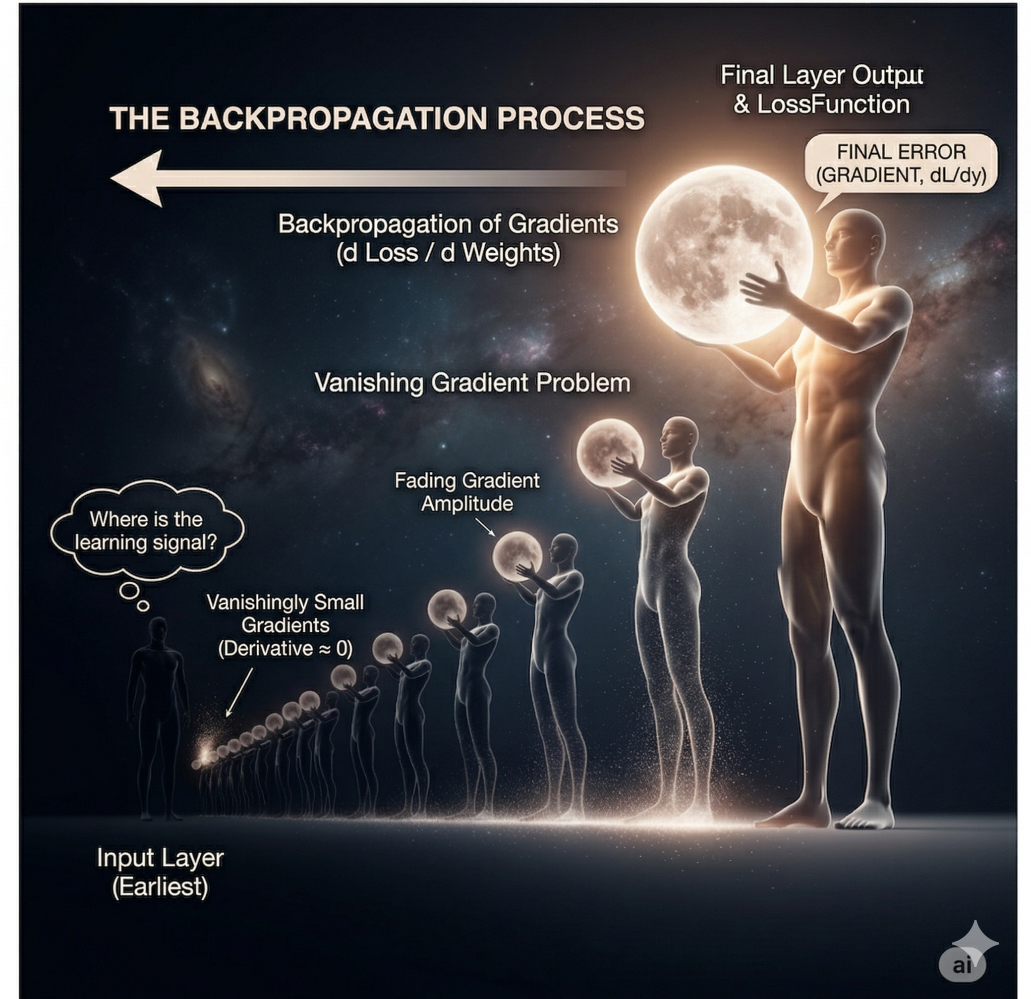
19. Vanishing Gradient Problem
The "Telephone Game" Problem
During training, the learning signal (gradient) must travel backward through all layers. But with each layer, it gets weaker and weaker until it vanishes into nothing.
Remember the "telephone game" where a message gets garbled as it passes through many people? Same problem here!
This roadblock stalled deep learning for decades. Modern fixes like ReLU activations and LSTM cells finally cracked it.

20. GANs: A Creative Duel
Generative Adversarial Networks
Ian Goodfellow's 2014 breakthrough: teaching AI to create by making two neural networks compete against each other!
- Generator (The Forger): Creates synthetic data trying to pass as real.
- Discriminator (The Detective): Tries to spot the fakes from the real deal.

21. The Training Arms Race
How They Improve Together
Round 1: Generator creates a crude blob. Discriminator easily spots it as fake.
After thousands of rounds: Generator gets better at faking. Discriminator sharpens its detection. Eventually, the fakes become indistinguishable from reality!
The Dark Side
- Deepfakes: Frighteningly realistic fake videos that can manipulate public opinion.
- Mode Collapse: Sometimes the generator gets stuck creating variations of the same thing over and over.
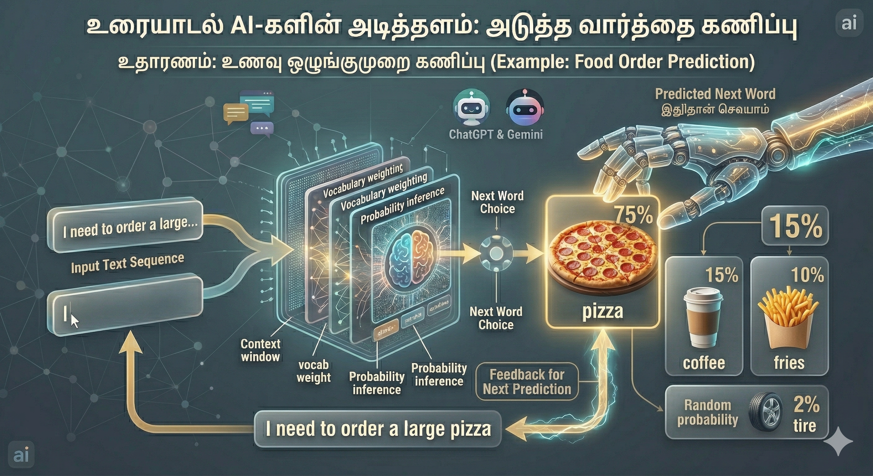
22. Transformers & Large Language Models
The architecture powering ChatGPT, Gemini, and the AI writing revolution.
- Next-Token Prediction: At its core, it's just predicting the next word based on what came before. Simple idea, profound results.
- Attention Mechanism: The breakthrough that lets AI understand context. It learns which words to "pay attention to".
Example: In "The animal didn't cross the street because it was too tired", attention helps determine "it" refers to the animal, not the street.